Catchment (TriMesh) [Py]

A simple example simulating the evolution of a single synthetic catchment on a triangular (irregular) mesh.

The local rate of elevation change, \(\partial h/\partial t\), is governed by bedrock river channel erosion (stream-power law).

(1)\[\frac{\partial h}{\partial t} = - K_f A^m (\nabla h)^n\]

where \(A\) is the drainage area (i.e., the total upslope area from which the water flow converges) and \(K_f\), \(m\) and \(n\) are parameters (uniform in space and time).

The initial topography is a nearly flat plateau of a given elevation. The base level (catchment outlet) is lowered during the simulation at a constant rate.

import numpy as np
import matplotlib.pyplot as plt
import matplotlib.tri as mpltri
import pygalmesh

import fastscapelib as fs

Setup the Mesh, Flow Graph and Eroders

Import the coordinates of the catchment boundaries from a file and create a new irregular mesh (with quasi-uniform resolution) using a constrained triangulation algorithm available in the pygalmesh library.

basin_poly = np.load("basin.npy")
n_poly = basin_poly.shape[0]
constraints = list([list(s) for s in zip(range(n_poly), range(1, n_poly))])
constraints[-1][1] = 0

approx_resolution = 300.0

mesh = pygalmesh.generate_2d(
    basin_poly,
    constraints,
    max_edge_size=approx_resolution,
    num_lloyd_steps=2,
)

points = mesh.points
triangles = mesh.cells[0].data

Determine the base level node, which corresponds to the catchment outlet (a boundary node).

outlet_idx = np.argmax(points[:, 1])
base_levels = {outlet_idx: fs.NodeStatus.FIXED_VALUE}

Create a new TriMesh object and pass the existing mesh data.

grid = fs.TriMesh(points, triangles, base_levels)

Create a FlowGraph object with single direction flow routing and the resolution of closed depressions on the topographic surface. See Flow Routing Strategies for more examples on possible flow routing strategies.

By default, base level nodes are set from fixed value boundary conditions (the outlet node set above in this example).

flow_graph = fs.FlowGraph(grid, [fs.SingleFlowRouter(), fs.MSTSinkResolver()])

Setup the bedrock channel eroder with a given set of parameter values.

spl_eroder = fs.SPLEroder(
    flow_graph,
    k_coef=2e-4,
    area_exp=0.4,
    slope_exp=1,
    tolerance=1e-5,
)

Setup Initial Conditions and External Forcing

Create a flat (+ random perturbations) elevated surface topography as initial conditions. Also initialize the array for drainage area.

init_elevation = np.random.uniform(0, 1, size=grid.shape) + 500.0
elevation = init_elevation
drainage_area = np.empty_like(elevation)

The base level lowering rate:

lowering_rate = 1e-4

Run the Model

Run the model for one hundred time steps.

dt = 2e4
nsteps = 100

for step in range(100):
    # base level (outlet) lowering 
    elevation[outlet_idx] -= lowering_rate * dt
    
    # flow routing
    flow_graph.update_routes(elevation)
    
    # flow accumulation (drainage area)
    flow_graph.accumulate(drainage_area, 1.0)
    
    # channel erosion (SPL)
    spl_erosion = spl_eroder.erode(elevation, drainage_area, dt)
    
    # update topography
    elevation -= spl_erosion

Plot Outputs and Other Diagnostics

x, y = points.transpose()
plot_tri = mpltri.Triangulation(x, y, triangles)

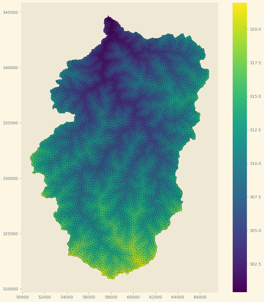
• Topographic elevation

fig, ax = plt.subplots(figsize=(13, 13))
ax.set_aspect('equal')
cf = ax.tripcolor(plot_tri, elevation)
plt.colorbar(cf)
ax.triplot(plot_tri, linewidth=0.2, c="k");

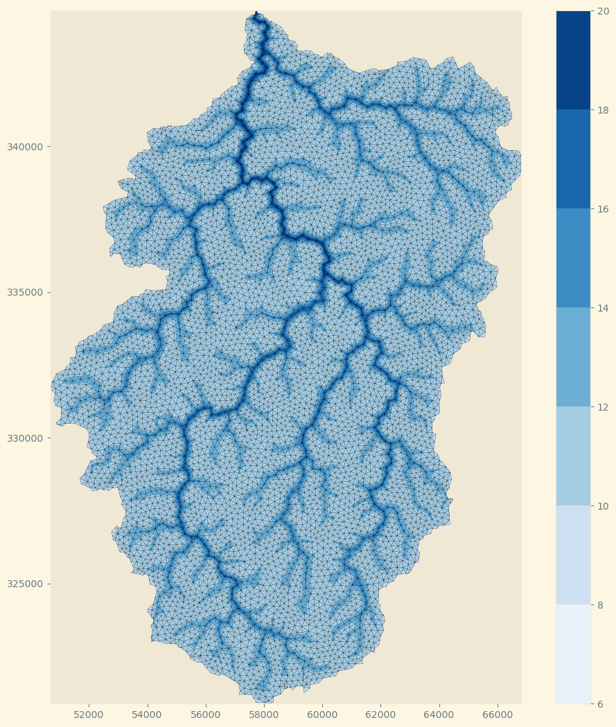
• Drainage area (log)

fig, ax = plt.subplots(figsize=(13, 13))
ax.set_aspect('equal')
cf = ax.tricontourf(plot_tri, np.log(drainage_area), cmap=plt.cm.Blues)
plt.colorbar(cf);
ax.triplot(plot_tri, linewidth=0.2, c="k");