River Profile [Py]
A simple example simulating the evolution of a river longitudinal profile under the action of block-uplift vs. bedrock channel erosion, starting from a very gentle channel slope. See also River Profile [C++].
The local rate of elevation change, \(\partial h/\partial t\), is determined by the balance between uplift (uniform in space and time) \(U\) and bedrock channel erosion modeled using the Stream-Power Law (SPL).
where \(A\) is the drainage area and \(K_f\), \(m\), \(n\) are SPL parameters (uniform in space and time).
import fastscapelib as fs
import numpy as np
import matplotlib.pyplot as plt
Setup the Grid, Flow Graph and Eroders
Create a ProfileGrid of 101 nodes each uniformly spaced by 300 meters.
Set fixed-value boundary conditions on the left side and free (core) conditions on the right side of the profile.
grid = fs.ProfileGrid(101, 300.0, [fs.NodeStatus.FIXED_VALUE, fs.NodeStatus.CORE])
Set x-coordinate values along the profile grid, which correspond to the distance from the ridge top. Start at x0 > 0 so that the channel head effectively starts at some distance away from the ridge top.
x0 = 300.0
length = (grid.size - 1) * grid.spacing
x = np.linspace(x0 + length, x0, num=grid.size)
Create a FlowGraph object with single direction flow routing (trivial case for a 1-dimensional profile).
By default, base level nodes are set from fixed value boundary conditions (left node in this example).
flow_graph = fs.FlowGraph(grid, [fs.SingleFlowRouter()])
Compute drainage area along the profile using Hack’s Law.
hack_coef = 6.69
hack_exp = 1.67

drainage_area = hack_coef * x**hack_exp
Setup the SPL eroder class with a given set of parameter values.
spl_eroder = fs.SPLEroder(
    flow_graph,
    k_coef=1e-4,
    area_exp=0.5,
    slope_exp=1,
    tolerance=1e-5,
)
Setup Initial Conditions and External Forcing
Create an initial river profile with a very gentle, uniform slope.
init_elevation = (length + x0 - x) * 1e-4
elevation = init_elevation
Set upflit rate as uniform (fixed value) along the profile except at the base level node (zero).
uplift_rate = np.full_like(x, 1e-3)
uplift_rate[0] = 0.
Run the Model
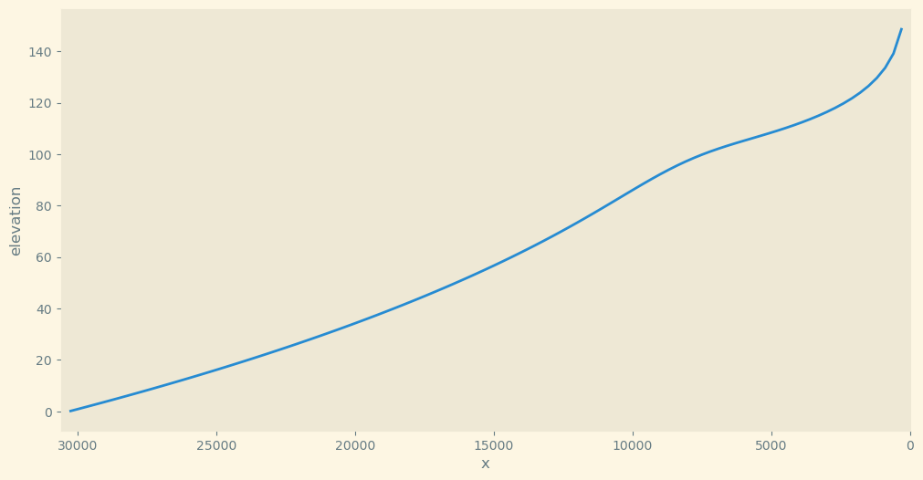
Run the model for a few thousands of time steps. At the middle of the simulation, change the value of the SPL coefficient to simulate a change in erodibility (e.g., climate change). This should create a knicpoint in the resulting river profile.
dt = 1e2
nsteps = 4000

# flow routing is required for solving SPL, although in this example
# it can be computed out of the time step loop since the
# flow path (single river) will not change during the simulation
# (not the case, e.g., if there were closed depressions!)
flow_graph.update_routes(elevation)


for step in range(nsteps):
    # uplift (no uplift at fixed elevation boundaries)
    uplifted_elevation = elevation + dt * uplift_rate

    # abrubpt change in erodibility
    if step == 3000:
        spl_eroder.k_coef /= 4

    # apply channel erosion
    spl_erosion = spl_eroder.erode(uplifted_elevation, drainage_area, dt)

    # update topography
    elevation = uplifted_elevation - spl_erosion
Plot the River Profile
fig, ax = plt.subplots(figsize=(12, 6))
ax.plot(x, elevation)
plt.setp(ax, xlabel="x", ylabel="elevation", xlim=(x[0] + 300.0, 0));