Mountain [Py]

A simple example simulating the formation of an orogenic belt (on a 2D raster grid) from a nearly-flat surface under the action of block-uplift vs. bedrock channel and hillslope erosion. See also Mountain [C++].

The local rate of elevation change, \(\partial h/\partial t\), is determined by the balance between uplift (uniform in space and time) \(U\) and erosion (stream-power law for river erosion and linear diffusion for hillslope erosion).

(1)\[\frac{\partial h}{\partial t} = U - K_f A^m (\nabla h)^n + K_D \nabla^2 h\]

where \(A\) is the drainage area (i.e., the total upslope area from which the water flow converges) and \(K_f\), \(m\), \(n\) and \(K_D\) are parameters (uniform in space and time).

The initial topography is nearly flat with small random perturbations and elevation remains fixed at the boundaries of the spatial domain.

from random import random

import fastscapelib as fs
import numpy as np
import matplotlib
import matplotlib.pyplot as plt

Setup the Grid, Flow Graph and Eroders

Create a RasterGrid of 201x301 nodes with a total length of 50 km in y (rows) and 75 km in x (columns).

Set fixed value boundary conditions at all border nodes.

grid = fs.RasterGrid.from_length([201, 301], [5e4, 7.5e4], fs.NodeStatus.FIXED_VALUE)

Create a FlowGraph object with single direction flow routing and the resolution of closed depressions on the topographic surface. See Flow Routing Strategies for more examples on possible flow routing strategies.

By default, base level nodes are set from fixed value boundary conditions (all border nodes in this example).

flow_graph = fs.FlowGraph(grid, [fs.SingleFlowRouter(), fs.MSTSinkResolver()])

Setup eroder classes (bedrock channel + hillslope) with a given set of parameter values.

spl_eroder = fs.SPLEroder(
    flow_graph,
    k_coef=2e-4,
    area_exp=0.4,
    slope_exp=1,
    tolerance=1e-5,
)

diffusion_eroder = fs.DiffusionADIEroder(grid, 0.01)

Setup Initial Conditions and External Forcing

Create a flat (+ random perturbations) surface topography as initial conditions. Also initialize the array for drainage area.

rng = np.random.Generator(np.random.PCG64(1234))

init_elevation = rng.uniform(0, 1, size=grid.shape)

elevation = init_elevation
drainage_area = np.empty_like(elevation)

Set upflit rate as uniform (fixed value) within the domain and to zero at all grid boundaries.

uplift_rate = np.full_like(elevation, 1e-3)
uplift_rate[[0, -1], :] = 0.
uplift_rate[:, [0, -1]] = 0.

Run the Model

Run the model for a few dozens of time steps (total simulation time: 1M years).

dt = 2e4
nsteps = 50

for step in range(nsteps):
    # uplift (no uplift at fixed elevation boundaries)
    uplifted_elevation = elevation + dt * uplift_rate
    
    # flow routing
    filled_elevation = flow_graph.update_routes(uplifted_elevation)
    
    # flow accumulation (drainage area)
    flow_graph.accumulate(drainage_area, 1.0)
    
    # apply channel erosion then hillslope diffusion
    spl_erosion = spl_eroder.erode(uplifted_elevation, drainage_area, dt)
    diff_erosion = diffusion_eroder.erode(uplifted_elevation - spl_erosion, dt)
    
    # update topography
    elevation = uplifted_elevation - spl_erosion - diff_erosion

Plot Outputs and Other Diagnostics

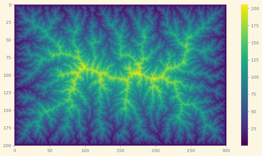
• Topographic elevation

fig, ax = plt.subplots(figsize=(12, 6))
plt.imshow(elevation)
plt.colorbar();

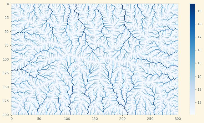
• Drainage area (log)

fig, ax = plt.subplots(figsize=(12, 6))
plt.imshow(np.log(drainage_area), cmap=plt.cm.Blues)
plt.colorbar();

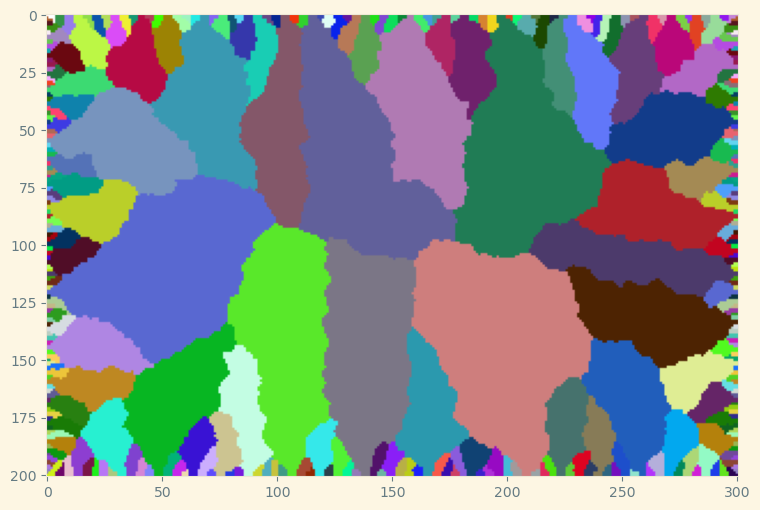
• Drainage basins

colors = [(1,1,1)] + [(random(),random(),random()) for i in range(255)]
rnd_cm = matplotlib.colors.LinearSegmentedColormap.from_list('new_map', colors, N=256)

fig, ax = plt.subplots(figsize=(12, 6))
plt.imshow(flow_graph.basins(), cmap=rnd_cm);