Inner Base Levels [Py]

An example very similar to Mountain [Py] but setting the base level nodes inside the raster grid instead of on the boundaries. The modeled domain is thus infinite (fully periodic), which is usefull for global (planetary) scale simulations.

from random import random, uniform

import fastscapelib as fs
import numpy as np
import matplotlib
import matplotlib.pyplot as plt

Setup the Grid, Flow Graph and Eroders

Create a RasterGrid of 201x201 nodes with a total length of 50 km in both y (rows) and x (columns).

Set looped (reflective) boundary conditions at all border nodes. Also set fixed-value “boundary” for a given number of base level nodes randomly selected inside the domain.

n_base_levels = 20
base_level_row = np.random.uniform(1, 200, n_base_levels).astype("int")
base_level_col = np.random.uniform(1, 200, n_base_levels).astype("int")

base_levels = {
    (i, j): fs.NodeStatus.FIXED_VALUE
    for i, j in zip(base_level_row, base_level_col)
}

bs = fs.NodeStatus.LOOPED
grid = fs.RasterGrid.from_length([201, 201], [5e4, 5e4], bs, base_levels)

Create a FlowGraph object with single direction flow routing and the resolution of closed depressions on the topographic surface. See Flow Routing Strategies for more examples on possible flow routing strategies.

By default, base level nodes are set from fixed value boundary conditions (random inner nodes in this example).

flow_graph = fs.FlowGraph(grid, [fs.SingleFlowRouter(), fs.MSTSinkResolver()])

Setup eroder classes (bedrock channel + hillslope) with a given set of parameter values.

spl_eroder = fs.SPLEroder(
    flow_graph,
    k_coef=2e-4,
    area_exp=0.4,
    slope_exp=1,
    tolerance=1e-5,
)

diffusion_eroder = fs.DiffusionADIEroder(grid, 0.01)

Setup Initial Conditions and External Forcing

Create a flat (+ random perturbations) surface topography as initial conditions. Also initialize the array for drainage area.

rng = np.random.Generator(np.random.PCG64(1234))

init_elevation = rng.uniform(0, 1, size=grid.shape)

elevation = init_elevation
drainage_area = np.empty_like(elevation)

Set upflit rate as uniform (fixed value) within the domain and to zero at all grid boundaries.

uplift_rate = np.where(
    grid.nodes_status() == fs.NodeStatus.FIXED_VALUE.value, 0, 1e-3
)

Run the Model

Run the model for a few dozens of time steps (total simulation time: 1M years).

dt = 2e4
nsteps = 50

for step in range(nsteps):
    # uplift (no uplift at fixed elevation boundaries)
    uplifted_elevation = elevation + dt * uplift_rate
    
    # flow routing
    filled_elevation = flow_graph.update_routes(uplifted_elevation)
    
    # flow accumulation (drainage area)
    flow_graph.accumulate(drainage_area, 1.0)
    
    # apply channel erosion then hillslope diffusion
    spl_erosion = spl_eroder.erode(uplifted_elevation, drainage_area, dt)
    diff_erosion = diffusion_eroder.erode(uplifted_elevation - spl_erosion, dt)
    
    # update topography
    elevation = uplifted_elevation - spl_erosion - diff_erosion

Plot Outputs and Other Diagnostics

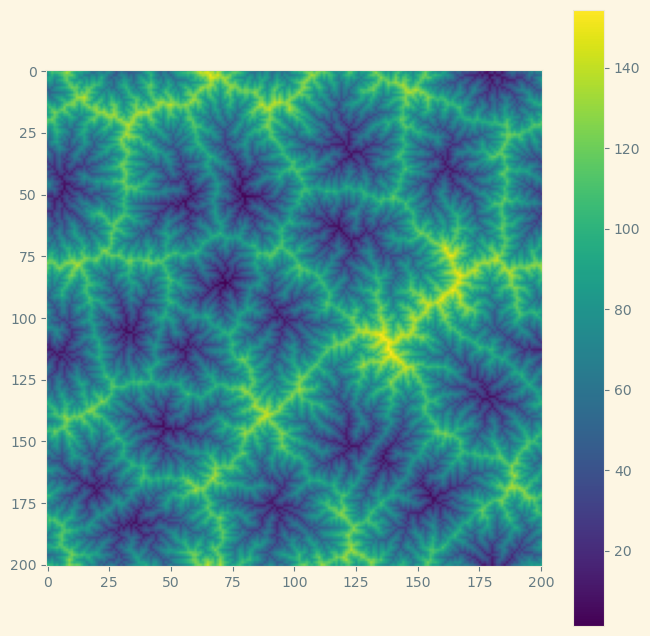
• Topographic elevation

fig, ax = plt.subplots(figsize=(8, 8))
plt.imshow(elevation)
plt.colorbar();

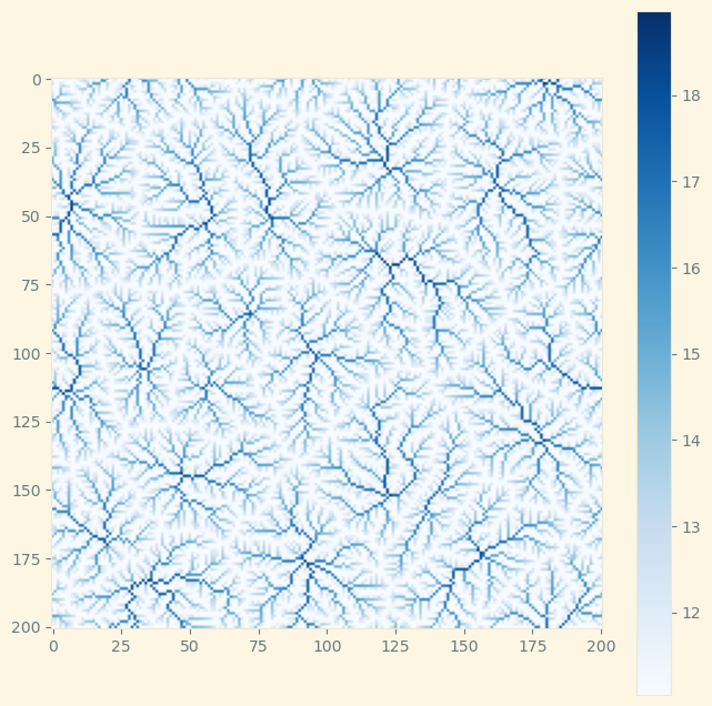
• Drainage area (log)

fig, ax = plt.subplots(figsize=(8, 8))
plt.imshow(np.log(drainage_area), cmap=plt.cm.Blues)
plt.colorbar();

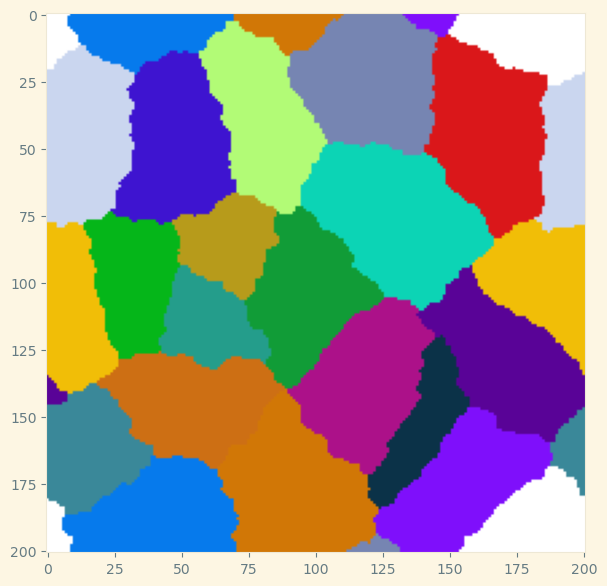
• Drainage basins

colors = [(1,1,1)] + [(random(),random(),random()) for i in range(255)]
rnd_cm = matplotlib.colors.LinearSegmentedColormap.from_list('new_map', colors, N=256)

fig, ax = plt.subplots(figsize=(7, 7))
plt.imshow(flow_graph.basins(), cmap=rnd_cm);