Planetary [Py]

A simple example simulating the evolution of a planet under the action of vertical uplift and bedrock channel erosion.

This example is pretty similar to Mountain [Py], although solving equation (1) without the hillslope linear diffusion term \(K_D \nabla^2 h\) on a spherical domain, leveraging Fastscapelib’s support for the HEALPix grid.

Note

Fastscapelib support for HEALPix is only available in the Linux and MacOS packages published on conda-forge.

import healpy as hp
import numpy as np
import matplotlib
import matplotlib.pyplot as plt

import fastscapelib as fs

# Theme that looks reasonably fine on both dark/light modes
matplotlib.style.use('Solarize_Light2')
matplotlib.rcParams['axes.grid'] = False

Setup the Grid, Flow Graph and Eroders

Create a HealpixGrid with a given value of nside, which corresponds to a number of refinement levels from the initial tessellation of the sphere. From this value we can compute the grid resolution and total number of nodes.

nside = 100

print("total nb. of nodes: ", hp.nside2npix(nside))
print("approx. resolution (km): ", hp.nside2resol(nside) * 6.371e3)

total nb. of nodes:  120000
approx. resolution (km):  65.19614456327078

As “boundary” conditions, we set a strip of a given width along the equator that will represent the planet’s ocean. This is done via the healpy library that allows handling HEALPix grids from within Python.

# set thin strips on each side from the equator (coastlines)
# with "FIXED VALUE" node status
nodes_status = np.zeros(hp.nside2npix(nside), dtype=np.uint8)
ocean_idx = hp.query_strip(nside, np.deg2rad(85), np.deg2rad(91))
nodes_status[ocean_idx] = fs.NodeStatus.FIXED_VALUE.value

# set "ghost" nodes between the two thin strips (ocean)
ocean_idx = hp.query_strip(nside, np.deg2rad(85.5), np.deg2rad(90.5))
nodes_status[ocean_idx] = fs.NodeStatus.GHOST.value

mask = nodes_status == fs.NodeStatus.GHOST.value

Create the grid object with a radius equal to the Earth’s radius.

grid = fs.HealpixGrid(nside, nodes_status, 6.371e6)

Create the flow graph and eroder objects. Set a mask for the flow graph from the “ocean” grid nodes.

flow_graph = fs.FlowGraph(
    grid,
    [fs.SingleFlowRouter(), fs.MSTSinkResolver()],
)
flow_graph.mask = mask

spl_eroder = fs.SPLEroder(
    flow_graph,
    k_coef=1.2e-11,
    area_exp=0.45,
    slope_exp=1,
    tolerance=1e-5,
)

urate = 9e-4

dt = 1e4

Create and Run a Simulation

Create a simple simulation runner.

def run_simulation(nsteps):
    rng = np.random.Generator(np.random.PCG64(123456789))
    init_elevation = rng.uniform(0, 1, size=grid.shape)
    elevation = init_elevation.copy()
    drainage_area = np.zeros_like(elevation)
    uplift_rate = np.full_like(elevation, urate)
    uplift_rate[grid.nodes_status() > fs.NodeStatus.CORE.value] = 0.

    for step in range(nsteps):
        uplifted_elevation = elevation + uplift_rate * dt
        
        # flow routing
        flow_graph.update_routes(uplifted_elevation)
        
        # flow accumulation (drainage area)
        flow_graph.accumulate(drainage_area, 1.0)
        
        # apply channel erosion then hillslope diffusion
        spl_erosion = spl_eroder.erode(uplifted_elevation, drainage_area, dt)
        
        # update topography
        elevation = uplifted_elevation - spl_erosion

    return elevation, drainage_area

Run the model for a few dozens of time steps (total simulation time: 400 000 years).

elevation, drainage_area = run_simulation(40)

Plot Outputs

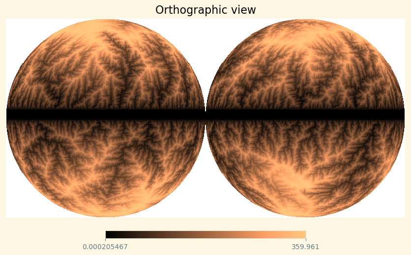
• Topographic elevation

hp.orthview(elevation, nest=False, cmap=plt.cm.copper)

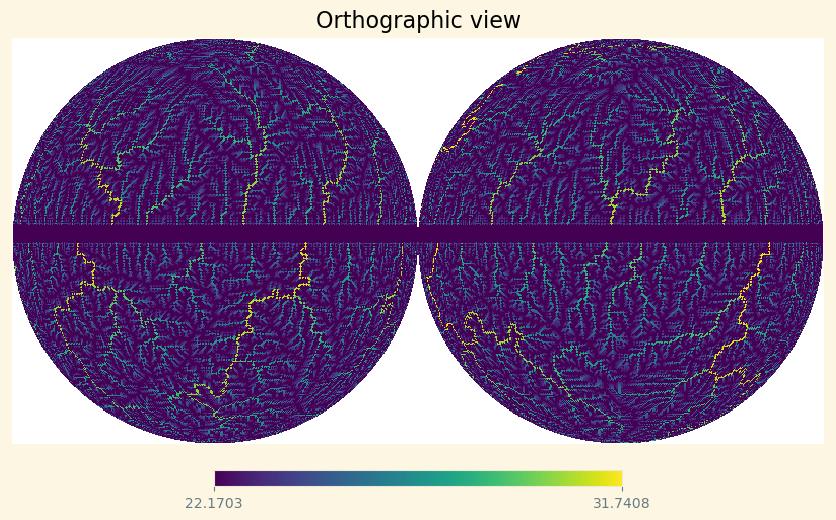
• Drainage area (log)

hp.orthview(np.log(drainage_area), nest=False);